We talked about Bayesian decision rule in
Chapter 3, in which we assumed that
x is a scalar or 1-dimension and we have known the exact density function. In reality, we have to make decision based on many criteria (so
x is a feature vector or high dimension) and we do not know the perfect and exact density function. The former problem that we addressed in
Chapter 4 and the latter will be considered in this chapter.
We have two methods to estimate function: Maximum-likelihood (MLE) and Maximum-A-Posterior (MAP). We will consider MLE in this chapter, the latter will be told in Chapter 6. The discriminant function in
Chapter 3:
It is easy to know

because it is
relative class frequencies, but

is difficult. To estimate the likelihood, we can predict the kind of density function (Gaussian, Poisson, Uniform distribution, ...) and estimate that function as well as use the resulting estimates (for more exact result, we should consider mixed densities as we told in
Chapter 2).
Because the unknown function
depends on a few parameters, so we transfer from the unknown-function estimating problem to the problem of estimating parameters of known-function. For example: Gaussian distribution we estimate mean(s) and (co-)variance.
1. Maximum-Likelihood estimate (MLE)
MLE is maximizing the likelihood (the probability of obtaining
the observed training samples). Informally interpreting, MLE chooses parameters to maximize as discriminant function in
Chapter 3. Let

is parameter vector of class

. For example, Gaussian density function (n-dimension):
Note that superscripts are not power of parameters, they illustrate
i-th dimension. Because

depends on

, so
=

. Because we observe over several samples, so we let
Di is training data, which contains samples of class
and transfer from maximizing

problem to maximizing

problem. Assume that
Di give no information about if
if , so the parameters for the
 different classes are independent (in case of dependent parameters, we can use
Hidden-Markov models). That is why we can work with each class
separately, and eliminate the notation of class distinctions . Now, our task is transferred from maximizingproblem to
maximizing
problem. Let
D contains n samples:
x1, x2, ..., xn. Since samples are independent, so:

(1)
MLE will estimate

by selecting optimal

having the highest probability
. Intuitively,
the value of  best agrees with the actually observed training sample:
(*Source: Richard O.Duda et al. Pattern Recognition)
This means we find gradient of distribution density over parameters and set this gradient to be equal 0:
Inserting (1) to above equation:
To be convenient for
analytical purposes, we will estimatewith the logarithm of the likelihood than with the likelihood itself (especially Gaussian distribution).
Maximum likelihood corresponds to minimum negative log-likelihood due to functional form of log-function and probability values between 0 and 1.

(2)
Because:
so (2):
Hence, the gradient of log-likelihood over parameters to be equal 0:

(3)
We will find optimal parametersfrom
(3) in the next parts with different distribution density functions.
2. MLE in Gaussian distribution (unknown mean)
We find optimal mean vector to maximize log-likelihood:
In general, we consider high-dimension Gaussian distribution:
Because the gradient of constant is 0, so we eliminate the first gradient:

(4)

(5)

(6)
We insert (5) and (6) to (4):
Where

is optimal mean vector. Since

is not
zero-matrix, so:
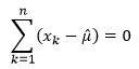
To achieve the maximum-likelihood, the mean vector is the arithmetic average of the training samples.
3. MLE in Gaussian distribution (unknown mean and covariance)
We will find the gradient of log-likelihood over mean vector and covariance. Since the analysis of the multi-variate case is basically very similar to uni-variate case, we will consider uni-variate case and predict the results in multi-variate case.
We obtain the results:
and
From the above results, we have the results in multi-variate:
and
Both results are arithmetic average or expected value.
4. MLE in Poisson distribution
Likelihood of Poisson distribution:
Log-likelihood is:
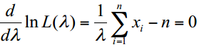
The derivative of log-likelihood over lambda is equal 0:
The optimal parameter is the arithmetic average:
5. Summary





 :
: