Pattern Recognition - Chapter 4: Discriminant function with Gaussian distribution

In Chapter 3, I introduced discriminant function, which choose the highest posterior probability distribution:

(1)

In Chapter 3, we assumed that x is a scalar or 1-dimension and we have known the exact density function. In reality, we have to make decision based on many criteria (so x is a feature vector or high dimension) and we do not know the perfect and exact density function. The latter problem that we will address in Chapter 5 and Chapter 6 and the former will be considered in this chapter. In this chapter, we will assume that the probabilities are normal distribution (high-dimension). Review on Chapter 2:

To simplify, we use logarithm of probability and remove the unimportant term (constants or the terms do not influence on the choosing of decision rule c(x)):

We will consider the different cases of covariance to have appropriate solution.

1. Independent features with the same (common) covariance

In this case, all discriminant function gi(x) have the same covariance and independent features or covariance matrix is diagonal matrix and the same variance.

From the above covariance formula, we have:

We apply logarithm and insert the above formula to (1):

We can eliminate , since it does not affect to choosing the optimal decision rule:

In the case of equal prior probabilities, we can eliminate prior probability and only decide the rule that make  minimum.  is Euclidean distance. As a result, we will assign observation x to the class which minimizes distance between observation vector and mean vector or minimum distance classifier.

(*Source: Tso B. and Mather P. Classification Methods for Remotely Sensed Data)

For example, the above figure illustrates Pixel a belonging to Class 1, because Class 1 is the nearest class.

However, in the case of inequality of prior probabilities, we will continue to expand . The term being inside arg max{.} is: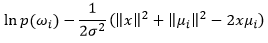

Because choosing of decision rule does not depend on , so we can eliminate . Finally, we have:

The final term, gained by letting the terms as coefficient, shows that when the features are independent with the common covariance, we will have linear discriminant function, which is linear separate (the boundary is hyper-plane). For this reason, we can apply linear perception or linear SVM to classify (see Machine Learning blog for detail information).

(*Source: Richard O.Duda et al. Pattern Recognition)

2. Dependent features with the same (common) covariance

In this case, all discriminant function gi(x) have the same covariance. We apply logarithm to (1):

We can eliminate , since it does not affect to choosing the optimal decision rule:

Since covariance matrix is symmetric; therefore, the inverse of covariance matrix is also symmetric. As a result, the transpose of the inverse covariance matrix:

As is a scalar, so it equals to its transpose:

, which leads to: 

Because of the properties of covariance matrix and the transpose of , the decision rule gi(x) equals to:

We can eliminate , since choosing of decision rule does not depend on it. We will obtain:

Consider the term, which is inside arg max{.}:

Again, the final term illustrates the features with the common covariance linear separate. For this reason, we can apply linear perception or linear SVM to discriminate.

3. Dependent features with the scaled covariance

In this case, all discriminant function gi(x) have the scaled covariance. From the above covariance formula, we have:

We apply logarithm and insert the above formula to (1):

Similar the second case, we gain:

Again, the term, which is inside arg max{.}, illustrates the features with the scaled covariance linear separate. For this reason, we can apply linear perception or linear SVM to discriminate:

4. Dependent features with the arbitrary covariance

We expand the logarithm of (1):

Unlike the first three cases, the features with arbitrary covariance is non-linear separate. Therefore, the boundary is conic- or  quadric-shape. To solve this problem, we use kernel trick (see Machine learning blog for more details) to transform data to higher dimension in which data can be linearly separated.

(*Source: Richard O.Duda et al. Pattern Recognition)