Pattern Recognition - Chapter 3: Bayes decision rule

To make the binary decision of  and  classes, we will choose the class which have the highest probability. In case of no observation of sample, we choose based on  and probabilities, known as prior probability. Because prior probability is overall probability considering over all dataset with very little information, so we always have the same decision for all samples. It is not meaning decision.
For above reason, we need an other criterion with observation of samples and more specific information to decide. The specific information will support us to make decision better such as temperature, humidity, cloudy level, ... for rain forecast, called as features. The support information is samples observation, which is the probability of the values of features, given class , or likelihood. The distribution of random variable x for class  is expressed in likelihood, which is gained by observation or survey. For example, how many female customers buy a Mercedes car, P(femal|Mercedes). To decide a class, it is necessary to have the probability of class , known a set of values of the features x: , the posterior probability. We should review Bayes rule in Chapter 1 to find posterior probability.

(*Source: Richard O.Duda et al. Pattern Recognition)

As above figure, we decide class  at x=14 since is highest. But this decision is always not correct, so we should consider error probability. Because this is binary decision, error probability is , which means the error occurs when  is true class and we choose . We decide class  because we want to minimize the error as possible.

1. Bayes decision rule

As above mention, it is necessary to consider error probability or risk function to make decision.

1.1. Risk function

It is difficult to have a complex risk function at this moment because we do not know the correct class and risk function need to consider over all samples. We will develop risk function from simple function, which is similar to Son Goku evolution in Dragon balls.

1.1.1. Simple cost function

This function looks like normal form of Son Goku. It is simple and easy to understand because we assume that we have known the correct class and fixed x (only one particular sample).

(*Source: http://www.writeups.org/songoku-age-23-dragon-ball/)

We will pay fee if we choose wrong class and it is free if the chosen class is correct:

(1)

where c(x) is the chosen class, given x and  is the correct class. However, we do not know the correct class, we need to evolve to other form of function.

1.1.2. Risk function depends the correct class

Son Goku evolves to the Super-Saiyajin 2.

(*Source: http://dragonballwiki.de/Son-Goku)

To address the correct-class-related problem, we will consider correct class as a random variable and compute risk function as an expected value of costs over all possible correct classes (review Chapter 1 for expected value computation).

(2)

The reason we use posterior probability in expected value of cost function is mentioned in introduction of this chapter. The above formular is denoted by R(c(x)|x). Note that x in this function is fixed (or a particular sample), but we need to consider over all samples, which is expanded in next part.

1.1.3. Risk function over all samples

Son Goku has evolved to the Super-Saiyajin 3.

(*Source:www.xemgame.com/ngoc-rong-dai-chien-khi-gioi-cosplay-dau-dau-voi-kieu-toc-cua-songoku-post144659.html)

As above mentioned, we will consider risk function over all samples (continous variables).

Similar to the above solution, we will consider feature vector x as random variable and compute risk function as an expected value of all possible x (again review Chapter 1 for expected value computation). But the problems are that x is continous random variable and x is a set of features, which means we will compute over high-dimension. To address the former, we replace sum by integral in the expected-value formular.

We insert R(c(x)|x) in (2) to the above:

(3)

This is a good way to transform from discrete variable to continous variable and a reason why mean computation is analogous to integral (I will illustrate its advantage in detail in Image processing blogs). For the latter problem - x is a feature vector (or high-dimension), we will handle in Chapter 4.

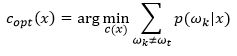
1.2. Bayes decision rule

As soon mentioned, the optimal classifier is minimizing the risk, which is (3). Choosing decision rule c(x) depends on x, does not depend on p(x). That is why we only minimize the term in (2).

Assume that  is the correct class (note that here is formular-development phrase, so we can assume the correct class):

The cost function of  class (correct class) is 0 and others are 1:

Because sum of probability is 1:

To minimize the term , we maximize :

(4)

This function, called MAP- Maximum A-Posterior, is used to make decision. In reality, given observation x, we compute posterior probability and choose the class with the highest probability. We will have the best decision if we have the correct posterior probability distribution (now we do still not know the exactly posterior probability distribution, which will be handled in the Chapter 5 and Chapter 6 by estimating the probability density function of parameters in this posterior probability distribution). Therefore, we transform classification problem to estimating the correct posterior probability distributions (MAP).

2. Discriminant functions and decision boundaries

2.1. Discriminant function

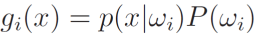
The useful and most prominent representation of a pattern classifier is discriminant functions gi(x).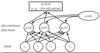

(*Source: Richard O.Duda et al. Pattern Recognition)

We will decide class if , or decide the class with the largest discriminant function, which is the highest posterior probability:

Note that we assume known posterior probability (estimating posterior probability - MLE or MAP will be considered in the Chapter 5 and Chapter 6). Using Bayes rule:

Or we can use logarithm of probability as a trick to avoid very small probability and to make easy when computing distribution (Gaussian distribution):

2.2. Decision boundary

If gi(x) > gj(x), we will decide class. How about gi(x) = gj(x)? This case if decision boundary, which means x is in decision boundary separating decision region.

(*Source: Richard O.Duda et al. Pattern Recognition)

In the chapter 4, we will consider in detail the probability of discriminant function (high-dimension).