Yesterday, I took part in the Bayesian network seminar, presented by Stefan Conrady in Munich. I have learned the interesting knowledge: Bayesian network.
(*Source: Stefan Conrady - Bayesian Network Presentation)
As I mentioned in
Chapter 1, Bayes rule illustrates the probability of dependent (and independent) probability, called conditional probability. In the real world, we have a lot of relationship factors, so the dependencies can be illustrated as networks, called Bayesian network.
For example, the result of exam influences on scholarship and my mood. The decision of going to bar based on scholarship (assume that I only gain money from scholarship) and my mood. If I go to bar, I would suit-up. Hence, from the above dependencies, I can build the network as the above picture.
The question is that why we need to use Bayesian network. Is it sexy? The answer is definitely "yes" (at least for my opinion).
1. Human and machine
In recent, many forums worry that the significant development of AI and Machine Learning leads the scenario that human under control by machines and robots. This could be because machine can learn easier and faster than human, especially human do not know what machine do or machine handle data as the blackbox. Bayesian network helps us to escape from this situation. There are interaction between human and machine during the process. Because human can understand through the network (see part 3), and it is understandable for machine to read network as the Directed Acyclic Graph.
(*Source: Stefan Conrady - Bayesian Network Presentation)
As the above figure, Machine Learning uses data to describe and predict the correlation. In contrast, human learns from theory to explain, simulate, optimize and attribute the causal relationship. The interaction between machine and human means machine describes and predicts from data (observation) and human then combine domain knowledge (part 2) to retrieve reasons (causal inference) through Bayesian network. Note that we cannot use data as reason (intervention), which will be explained in detail in part 5 through the example.
2. Compact the joint probability
One benefit we have when using Bayesian network is that reduce the unnecessary dependencies in joint probability. Back to the example of exam-clothes in introduction part, we have the joint probability:
p(exam,scholarship,mood,bar,suit-up) = p(suit-up|bar,scholarship,mood,exam) . p(bar|scholarship,mood,exam) . p(scholarship|mood,exam) . p(mood|exam)
Oops! It is so long and complicated! Imaging that what happens when we want to know the joint probability of 10,000 variables (example: the joint probability of dependent words).
To address this problem, we build Bayesian network by using domain knowledge, or our experience to reduce the dependencies (be careful with the difference between heuristic and biases). From my experience, the decision of suiting up does not involve to scholarship, my mood or the exam, and I will remove these dependencies. I continue to remove unnecessary dependencies:
p(exam,scholarship,mood,bar,suit-up) = p(suit-up|bar,scholarship,mood,exam) . p(bar|scholarship,mood,exam) . p(scholarship|mood,exam) . p(mood|exam)
Yeah! We cross out 5 dependencies from equation; therefore, the joint probability is compacted.
3. Formula visualization
I used to be very bad physics because of tons of formula that I need to remember. It was difficult to learn by heart all of them. I had an idea that I used graphs to illustrate the relationship between factors in formula. As a result, I understood and remembered these formula.Yesterday, I knew that I used to use Bayesian network to make formula easier to understand.
4. The curse of Dimensionality
In the 1D, 2D and 3D space, the nearer points have the lower distance. However, in the higher dimension, we can not use distance as the score to evaluate the nearest neighbors.
To explain it, we consider the distribution of A and B in D-dimension:
The distribution is the product of volume and average density of
x in region A:
The volume is proportional to Radius and Dimension, let
CD is the constant depends on number of dimension D:
Similar to region A, the density of region B:
Assume that the probability density in A is higher:
But
x is more likely to belong to region B if dimension
D=8:
This means
x belongs to A, being far away from center of distribution. As a consequence, the
distance measure, which becomes unreliable in higher dimensions.
Now, thanks to Bayesian network, we can compute its likelihood and avoid the distance measure.
5. Casual and Observational inference
I found that we are easily confused between observation and intervention. To be clearer, we will be back to the first example, I observe that my mood is influenced by the result of the exam. But now, there is no exam and I am rock-on, this means I do: p(mood=rock-on) = 100%
This confusion leads to a problem that I mentioned earlier in part 2 that we should not use the prediction from data as a reason. Here is an example to explain:
I will get the example in the presentation of Stefan Conrady on Bayesian network. People realized that the price of house will be proportional to the number of garages by linear regression:
(*Source: Stefan Conrady - Bayesian Network Presentation)
The wise owner thought that if he add two more garages, he would gain more $142,000.
(*Source: Stefan Conrady - Bayesian Network Presentation)
Oops!!! In fact the price of house does not increase since he did not observe, he did or intervene.
In the reality, we easily meet these faults as confounder, which makes mistakes in decision making especially medicine. For example: the doctor made a survey that coffee drinking causes lung cancer and concluded that coffee were not good for our lungs. But he did not that the coffee-aholic persons tend to smoke, which causes lung cancer.
Beside that, as Simpson's paradox, there are positive trends of variables in variety of groups, but the trend will be reversed when combining. This problem is caused by causal interpretation. For example: I assume data from some supermarket:
As above table, there is a conclusion that male customers tend to buy more than female. However, we consider the report for each store, it is very weird:
Looking at the above table, almost female customers tend to buy the goods in the stores which have fewer visitors. This is causal interpretation.
To sum up, correlation does not causation. Simpson's paradox points out that the correlation of two variables are positive, but in fact they are negatively correlated by the "lurking" confounder. Here is not artificial intelligence, that is human intelligence. That is why we need to combine artificial intelligence and human intelligence, which can be done via Bayesian network.

 that make likelihood maximum, meaning parameters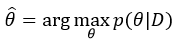


 .
.  and
and  are hyper-parameters.





 (1)
(1) as the true mean and
  as the true variance:
 (2)
(2)
 , with


 plays as the role of the prior. This means that Bayesian learning can improve the estimation of parameters by adding more observation.


