Pattern Recognition - Chapter 6: Bayesian parameter estimation

1. Introduce Bayesian parameter estimation (Maximum-A-posterior)

We talked about Bayesian decision rule in Chapter 3, in which we assumed that x is a scalar or 1-dimension and we have known the exact density function. In reality, we have to make decision based on many criteria (so x is a feature vector or high dimension) and we do not know the perfect and exact density function. The former problem that we addressed in Chapter 4 and the latter would be considered in Chapter 5 and this chapter.

As I mentioned in Chapter 5, to estimate the distribution we should maximize likelihood:

However, we assumed that we choose parameters  that make likelihood maximum, meaning parameters  are fixed. In reality, parameters are distributed as some distribution (e.g. Gaussian distribution), and we consider parameters as random variables: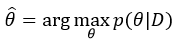

Expand posterior probability:

Because p(D) is independent on parameters, we consider this prior as a constant:

We can eliminate constant in max operation:

Look back into MLE:

Bayesian parameter estimation has additional information: prior probability as the weights. This means the prior knowledge will tune the important level of what we observed.

2. An example

I assume that the mean is unknown and is distributed as Gaussian distribution (known variance). We have two periods: pre- and post-observation.

2.1. The pre-observation

In this period, our knowledge on parameters is a Gaussian distribution, or .  and  are hyper-parameters.  is the best knowledge before observation and  is uncertainty.

2.2. The post-observation

After observing data D, the posterior is expanded:

We continue to expand prior and posterior:

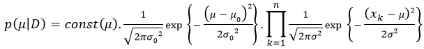
Let const' as new constant of posterior:

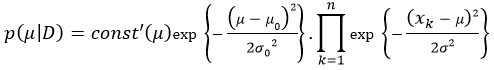
As exp{a}.exp{b} = exp{a+b}, so:

We continue to expand:

The term in the red rectangle is independent on mean, so we consider this term as constant:

(1)

As Chapter 2 mentioned, the product of two Gaussian distributions is a Gaussian distribution. We let  as the true mean and as the true variance:

(2)

From (1) and (2), we can have:

, with  

From above equation, the number of samples determines the importance of empirical mean and prior mean. The larger the number of sample is, the more important observation is.

3. Bayes learning

Bayesian parameter estimation:

Because of additional knowledge - the prior, we can utilize the prior to learn incrementally. This means that we can improve parameter estimation by increasing observations in spite of a few data in the initial phrase.

Assume that:

The posterior:

Because:

So we have:

In the above equation,  plays as the role of the prior. This means that Bayesian learning can improve the estimation of parameters by adding more observation.