Three basic functions in functional programming (Python)

There are three functions that facilitate functional programming: map, filter and reduce. To explain three functions, I will tell you story about Snow White and the seven Dwarfs. Of course, almost children know this fairy story, but do you know what the seven Dwarfs do? They mine ores, and I will tell you about their work.

1. Excavation - mapping

At the first stage, Each Dwarf excavate the surface of the rock and get potential ores. The mapping is a function as excavation of Dwarfs. Map applies a function (excavation) to all items in an input list (the surface of the rock) and return an same-size output list (ores in the carts).

Example:

   def add_one(x):

    return (x+1)

items = [1, 2, 3, 4, 5]
result = list(map(add_one, items))

Output: [2, 3, 4, 5, 6]

2. Filtering

After collecting the small pieces of rock, they remove scree and keep gemstone from the carts. The filter function also filters based on a specific condition (whether it is gemstone?), which removes elements (scree) that do not satisfy the condition and keeps elements (gemstone) that satisfy the condition.

Example:

   def is_even(x):

    return (x%2) == 0

items = [1, 2, 3, 4, 5]
result = list(filter(is_even, items))

Output: [2, 4]

3. Loading - Reduce

The night is coming, and seven dwarfs put gems into carts to bring to warehouse. They use connector to bridge cart each other and load to warehouse.

The 'Reduce' function is similar the seven dwarfs' work. This function performs 'rolling' computation (connect a pair of carts as a chain) on sequential pairs in the input list (pair of carts) and returns the result (put gems to the warehouse).

Example:

 def sum(x,y):

    return (x + y)

items = [1, 2, 3, 4, 5]
result = reduce(sum, items)

Output: 15

Optimize code for Parallel Processing

1. Parallel strategies

In the age of internet, computers need to process big data and the problem here is reduce running time. To reduce running time, we use parallel processing. There are three parallel strategies: pipeline, parallel data processing and simultaneous processing.

1.1. Pipeline

Firstly, pipeline is a strategy that is similar to product chain in the mill, which divides to many phrases. Output(phrase A) = Input(phrase B). We can see the procedure of the brick production chain in the below pictures:

Digger supplies the clay for the crusher to break up clay into smaller pieces. After supplying, digger goes on his jobs.

1.2. Parallel data processing

In this strategy, we use many processors to work the same jobs on different data, instead of phrases in pipeline.

(*Source: https://www.toonpool.com/cartoons/ANTS_143334)

As we can see the above pictures, the different ants brings various stuff, but the same operator is "BRING".

1.3. Simultaneous processing

Unlike to parallel data processing, the simultaneous processing uses processors to work the different jobs on different data.

(*Source: http://smurfs.wikia.com/wiki/Village_Smurphony_Orchestra)

Each artist in the orchestra plays the different instrument (different jobs) on different music sheet (different data).

2. Parallel models

We review on parallel strategies, but how to manage (control) the parallel process if we apply those parallel strategies. Basically, there are two models: working pool and master-slave.

2.1. Master-slave

Master-slave model requires a master to assign the duty to their workers. We can apply simultaneous processing to this model.

(*Source: https://i.ytimg.com/vi/-WGBFcZaT_M/maxresdefault.jpg)

2.2. Working pool

Processors in this model are free to choose data to handle (it look like you feel free to select products when shopping!!!). We frequently apply parallel data processing to this model.

(*Source: https://i.ytimg.com/vi/nhtJfhzM5iU/maxresdefault.jpg)

Sometimes we can apply simultaneous processing to this model, which is "Mixture of expert" (Ensemble model) in Machine learning. They use gating model (trained by Expectation-Maximization) to weight which learning machine (different job) is appropriate (dominant) to different data because there is no learning machine being better than others on full data (as "No free lunch" theorem).

(*Source: Sungmin Myoung, Modified Mixture of Experts for the Diagnosis of Perfusion Magnetic Resonance Imaging Measures in Locally Rectal Cancer Patients)

3. Optimize code for parallel processing

A question is that how we can apply parallel processing. The answer is that it is difficult to apply for the mutual-dependent data (pipeline is acceptable, but in some extend) and easy to handle the independent data as parallel processing. That is why we need to have ability to optimize code, which are pre-allocating array and vectorizing loops.

3.1. Pre-allocating array

We often use "append" operator on array, but it is not good because of memory fragmentation. For example, at the first stage, array A (six elements) was allocated at the first address, after some operations, appending two new elements to this array. Logically, we have a continuous 8-element array, but in physic memory, it looks like:

System will spend time to find the fragmented elements, which is time-consuming. To address this problem, we should predefine array size as possible to avoid fragmentation.

3.2. Vectorizing loops

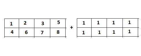
We should convert some for (while) loops to matrix operations. Here is an easy example:

We plus eight numbers to array at the same time instead of sequentially adding. This is equivalent to:

Now, we consider a more complex example. The example is that we swap two columns, i and j. The first thing comes to our mind is that we create a temporary vector to save values of column i, and then copy values of column j to column i. Finally, we copy values from temporary vector to column j.

But, what happens if we swap a thousand of columns? This method runs very slowly. Alternative, we use permutation matrix P to address this problem. If we want to swap columns, PxA; in the case of swapping rows, AxP. The permutation matrix is created by swapping identity matrix I. In below figure, we want to swap the first column and second column, so we swap the first column of I and the second column of I.

We continue to consider the next example. This is kernel problem, which is a popular and useful trick in machine learning and image processing. The kernel will slice on matrix from pixel to pixel as below figures.

Actually, kernel approach is sum of weighted neighbours' values. To implement as parallel process, we extract and stretch each region in matrix and kernel into column and dot-product column extracted from kernel to columns extracted from matrix.