Explanation of self-attention (single head)

Attention (*Source: https://jasperwalshe.com/perspective-and-performance/)

1. Main ideas

Convolutional neural networks (CNN) only focus on local dependencies using kernel (the pink area as Figure 1), and dependent information (green pixel as Figure 1) beyond the range of kernel will be not considered. To take into account long dependencies, there are Recurrent neural networks (RNN). However, the stream of previous information are controlled by gates, so integrated information are include irrelevant information and relevant information are faded. Researcher suggested Bi-LSTM, or reversed the order of stream (Senquence-2-sequence) to mitigate this issue. Another suggestion is self-attention network (SAN) that takes into account global dependencies (except from limited-SAN that consider in the fixed range to reduce memory-consumption).

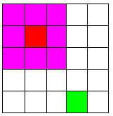
Figure 1. The dependent pixel is outside of the range of kernel in CNN.

The main idea of SAN is based on query-key-value. Think of dictionary in Python (or HashTable in Java). There are pairs of key-value as Figure 2. To retrieve information (value), user sends the query to machine. Machine lookup then all keys, choose the key which is exactly matched the query and retrieve corresponding value to respond user's request. As the Figure 2.a, the query of "water" is exactly matched the key of "water". Therefore, the information should be 100%*28.

Figure 2. Retrieve information by query-key. a. Query is exactly matched key. b. Query likely is matched key.

Likely, SAN will match query to key to determine which information are retrieved. However, it is, in practice, difficult to match exactly. Hence, SAN measures relationship between query and key that implies how likely the information that user needs. In the other words, this mechanism are considered as gate in RNN (but no matter of the locations of query and key). As Figure 2.b, the query of "H2O" is 80% matched the key of "water" and 20% matched the key of "rain". Hence, the information should be 80%*28 + 20%*46 = 31.6.

Figure 3. The model of Attention (single-head)

2. Architecture

As Figure 3, there are three main parts in the model of SAN: Linear transformation input (input becomes key, value and query via linear transformation), similarity calculation and weighted sum.

Firstly, why are there linear transformation? Their weights are trainable variables that learn the way to transform to new coordinates in which the dependencies are "visible" or easy to extract. Second reason is that linear transformation make sure new features (known as head) representing various aspects such that enriches diversity in the case of multi-head attention (each head represent a particular aspect). Note that, the weights in transformations of query, key and value are not shared variables. The below code show linear transformation.

# linear transformation
trans_k = tf.layers.dense(key_, args['n_hid_channel'])
trans_q = tf.layers.dense(query_, args['n_hid_channel'])
trans_v = tf.layers.dense(value_, args['n_in_channel'])

Of course, the value is the intensity of vector (gray level - Image Processing, word embedding - NLP or intensity of spectrum - Speech processing). Next, the similarity between key and query is the relationship between two locations in feature vector (a pixel - Image Processing, an embedding feature - NLP or a wave channel - Speech Processing). Here, SAN considers the intensity to be a metric to measure the level of relationship. Therefore, the input are became key, query and value after non-sharing linear transformation.

But, how to measure the above relationship? Self-attention uses dot-product to illustrate relationship or distance between key and query. The question is: Why dot-product?

Think about cosine distance. This distance measures the difference of angle as Figure 4, and the formula is in Equation 1.

Figure 4. Illustration of cosine distance. (*Source: https://www.machinelearningplus.com/nlp/cosine-similarity/)

Equation 1. Cosine distance.

The aim is that using cosine distance to measure similarity between key and query. We consider key and query as two vectors in the space. As Equation 1, cosine distance is dot product between two vectors (key and query), followed by normalization by their magnitudes. From that, cosine distance is equivalent to matrix multiplication, followed by sigmoid function. Hence, to convert to matrix operation, SAN firstly uses matrix multiplication which measure angle distance without normalization. SAN then normalizes this distance by using sigmoid function to generate value in the range of [0,1] (Sigmoid is consider as the gate that controls how much value is released).

# find dependencies using multiply of keys and queries
depend = tf.matmul(trans_q, trans_k, transpose_b=True)

# find similarity using softmax of dependencies

similarity = tf.nn.softmax(depend)

Finally, integrated information is weighted sum of value by using matrix multiplication between similarity coefficient and value.

# find head by multiply similarity by values

head = tf.matmul(similarity, trans_v)

To sum up, we will receive a new feature vector from input. However, this vector (head) only represents one aspect of global dependencies. To make it more diverse, we should use multi-head attention. I will cover this issue in the next blog.
Full code here: https://github.com/nhuthai/Feature-learning/tree/master/SAN

3. References

A. Vaswani, N. Shazeer, N. Parmar, J. Uszkoreit, L. Jones, A. N. Gomez, L. Kaiser, I. Polosukhin, Attention is all you need. in NIPS 2017, 2017.

Pattern Recognition - Chapter 6: Bayesian parameter estimation

1. Introduce Bayesian parameter estimation (Maximum-A-posterior)

We talked about Bayesian decision rule in Chapter 3, in which we assumed that x is a scalar or 1-dimension and we have known the exact density function. In reality, we have to make decision based on many criteria (so x is a feature vector or high dimension) and we do not know the perfect and exact density function. The former problem that we addressed in Chapter 4 and the latter would be considered in Chapter 5 and this chapter.

As I mentioned in Chapter 5, to estimate the distribution we should maximize likelihood:

However, we assumed that we choose parameters  that make likelihood maximum, meaning parameters  are fixed. In reality, parameters are distributed as some distribution (e.g. Gaussian distribution), and we consider parameters as random variables:

Expand posterior probability:

Because p(D) is independent on parameters, we consider this prior as a constant:

We can eliminate constant in max operation:

Look back into MLE:

Bayesian parameter estimation has additional information: prior probability as the weights. This means the prior knowledge will tune the important level of what we observed.

2. An example

I assume that the mean is unknown and is distributed as Gaussian distribution (known variance). We have two periods: pre- and post-observation.

2.1. The pre-observation

In this period, our knowledge on parameters is a Gaussian distribution, or .  and  are hyper-parameters.  is the best knowledge before observation and  is uncertainty.

2.2. The post-observation

After observing data D, the posterior is expanded:

We continue to expand prior and posterior:

Let const' as new constant of posterior:

As exp{a}.exp{b} = exp{a+b}, so:

We continue to expand:

The term in the red rectangle is independent on mean, so we consider this term as constant:

(1)

As Chapter 2 mentioned, the product of two Gaussian distributions is a Gaussian distribution. We let  as the true mean and as the true variance:

(2)

From (1) and (2), we can have:

, with  

From above equation, the number of samples determines the importance of empirical mean and prior mean. The larger the number of sample is, the more important observation is.

3. Bayes learning

Bayesian parameter estimation:

Because of additional knowledge - the prior, we can utilize the prior to learn incrementally. This means that we can improve parameter estimation by increasing observations in spite of a few data in the initial phrase.

Assume that:

The posterior:

Because:

So we have:

In the above equation,  plays as the role of the prior. This means that Bayesian learning can improve the estimation of parameters by adding more observation.

Introduce Bayesian network

Yesterday, I took part in the Bayesian network seminar, presented by Stefan Conrady in Munich. I have learned the interesting knowledge: Bayesian network.

(*Source: Stefan Conrady - Bayesian Network Presentation)

As I mentioned in Chapter 1, Bayes rule illustrates the probability of dependent (and independent) probability, called conditional probability. In the real world, we have a lot of relationship factors, so the dependencies can be illustrated as networks, called Bayesian network.

For example, the result of exam influences on scholarship and my mood. The decision of going to bar based on scholarship (assume that I only gain money from scholarship) and my mood. If I go to bar, I would suit-up. Hence, from the above dependencies, I can build the network as the above picture.
The question is that why we need to use Bayesian network. Is it sexy? The answer is definitely "yes" (at least for my opinion).

1. Human and machine

In recent, many forums worry that the significant development of AI and Machine Learning leads the scenario that human under control by machines and robots. This could be because machine can learn easier and faster than human, especially human do not know what machine do or machine handle data as the blackbox. Bayesian network helps us to escape from this situation. There are interaction between human and machine during the process. Because human can understand through the network (see part 3), and it is understandable for machine to read network as the Directed Acyclic Graph.

(*Source: Stefan Conrady - Bayesian Network Presentation)

As the above figure, Machine Learning uses data to describe and predict the correlation. In contrast, human learns from theory to explain, simulate, optimize and attribute the causal relationship. The interaction between machine and human means machine describes and predicts from data (observation) and human then combine domain knowledge (part 2) to retrieve reasons (causal inference) through Bayesian network. Note that we cannot use data as reason (intervention), which will be explained in detail in part 5 through the example.

2. Compact the joint probability

One benefit we have when using Bayesian network is that reduce the unnecessary dependencies in joint probability. Back to the example of exam-clothes in introduction part, we have the joint probability:

p(exam,scholarship,mood,bar,suit-up) = p(suit-up|bar,scholarship,mood,exam) .  p(bar|scholarship,mood,exam) . p(scholarship|mood,exam) .  p(mood|exam)

Oops! It is so long and complicated! Imaging that what happens when we want to know the joint probability of 10,000 variables (example: the joint probability of dependent words).

To address this problem, we build Bayesian network by using domain knowledge, or our experience to reduce the dependencies (be careful with the difference between heuristic and biases). From my experience, the decision of suiting up does not involve to scholarship, my mood or the exam, and I will remove these dependencies. I continue to remove unnecessary dependencies:

p(exam,scholarship,mood,bar,suit-up) = p(suit-up|bar,scholarship,mood,exam) .  p(bar|scholarship,mood,exam) . p(scholarship|mood,exam) .  p(mood|exam)

Yeah! We cross out 5 dependencies from equation; therefore, the joint probability is compacted.

3. Formula visualization

I used to be very bad physics because of tons of formula that I need to remember. It was difficult to learn by heart all of them. I had an idea that I used graphs to illustrate the relationship between factors in formula. As a result, I understood and remembered these formula.Yesterday, I knew that I used to use Bayesian network to make formula easier to understand.

4. The curse of Dimensionality

In the 1D, 2D and 3D space, the nearer points have the lower distance. However, in the higher dimension, we can not use distance as the score to evaluate the nearest neighbors.
To explain it, we consider the distribution of A and B in D-dimension:

The distribution is the product of volume and average density of x in region A:

The volume is proportional to Radius and Dimension, let CD is the constant depends on number of dimension D:

Similar to region A, the density of region B:

Assume that the probability density in A is higher:

But x is more likely to belong to region B if dimension D=8:

This means x belongs to A, being far away from center of distribution. As a consequence, the distance measure, which becomes unreliable in higher dimensions.
Now, thanks to Bayesian network, we can compute its likelihood and avoid the distance measure.

5. Casual and Observational inference

I found that we are easily confused between observation and intervention. To be clearer, we will be back to the first example, I observe that my mood is influenced by the result of the exam. But now, there is no exam and I am rock-on, this means I do: p(mood=rock-on) = 100%

This confusion leads to a problem that I mentioned earlier in part 2 that we should not use the prediction from data as a reason. Here is an example to explain:

I will get the example in the presentation of Stefan Conrady on Bayesian network. People realized that the price of house will be proportional to the number of garages by linear regression:

(*Source: Stefan Conrady - Bayesian Network Presentation)

The wise owner thought that if he add two more garages, he would gain more $142,000.

(*Source: Stefan Conrady - Bayesian Network Presentation)

Oops!!! In fact the price of house does not increase since he did not observe, he did or intervene.

In the reality, we easily meet these faults as confounder, which makes mistakes in decision making especially medicine. For example: the doctor made a survey that coffee drinking causes lung cancer and concluded that coffee were not good for our lungs. But he did not that the coffee-aholic persons tend to smoke, which causes lung cancer.

Beside that, as Simpson's paradox, there are positive trends of variables in variety of groups, but the trend will be reversed when combining. This problem is caused by causal interpretation. For example: I assume data from some supermarket:

As above table, there is a conclusion that male customers tend to buy more than female. However, we consider the report for each store, it is very weird:

Looking at the above table, almost female customers tend to buy the goods in the stores which have fewer visitors. This is causal interpretation. 

To sum up, correlation does not causation. Simpson's paradox points out that the correlation of two variables are positive, but in fact they are negatively correlated by the "lurking" confounder. Here is not artificial intelligence, that is human intelligence. That is why we need to combine artificial intelligence and human intelligence, which can be done via Bayesian network.